Last year we released NAP v0.5.0 which completely revamped the look and feel of the platform and introduced lots of new features and improvements. The update included a powerful addition to our Vulkan render engine that had been on my wishlist for a while; Compute support! This finally gives NAP apps the tools to access general purpose computing on the GPU optimized for applications beyond rendering. We thought now would be a good time to explain the abstraction in more detail and demonstrate how we have been using it in our projects.

Vulkan Compute lets you compose and command arbitrary GPU workloads using a simplified compute pipeline, as opposed to the graphics pipeline. This means you can execute shader programs without the typical overhead of processing graphics; the extensive set of fixed and programmable stages (input assembly, vertex, tesselation, fragment, rasterization etc.), but also lots of specialized API calls and synchronization methods. The compute pipeline, conversely, is simple in that it consists of a single programmable stage for processing a compute shader, and a smaller, less complicated subset of API calls to work with. All this makes compute pipelines more flexible and better suitable for tasks such as mesh and texture manipulation, procedural generation, particle simulations, GPU acceleration structures (e.g. visibility culling) and much more.
Naturally, with growing adoption of NAP and increasingly demanding projects on our side, support for Vulkan Compute grants us many new possibilities.

The Vulkan Compute abstraction is designed such that the exposed functionality fits neatly into NAP's data-driven paradigm and workflow. This means users must be able to formulate compute work by means of modular building blocks; resources, components, entities as well as dependencies between them, in data.
Existing NAP concepts for shaders and materials always assumed the graphics pipeline. Therefore, the update introduces base classes for both to distinguish between graphics and compute variants (with future extensions in mind). We now consider any material (nap::BaseMaterial) to be no more than an aggregation of three types of resource bindings; uniforms, textures and buffers. The derived class for a graphics material (nap::Material) includes an additional resource type for vertex attribute bindings, and blend/depth mode flags.
If you are already familiar with the existing NAP workflow for rendering graphics you will recognize a few conventions:
nap::ComputeShader loads and compiles a compute shader program (analogous to nap::Shader)nap::ComputeMaterial creates compute shaders resource bindings (analogous to nap::Material)nap::ComputeComponent sets up and dispatches the compute program (analogous to nap::RenderComponent)At a lower level, we can distinguish compute pipelines by their shader program alone. This introduces nap::ComputePipelineKey to fetch the appropriate compute pipeline from the nap::RenderService::ComputePipelineCache (analogous to nap::PipelineKey and nap::RenderService::PipelineCache).
Some modifications were made to nap::RenderService to create and manage a dedicated compute queue vkQueue and compute command buffer vkCommandBuffer per frame in flight.
I also introduced nap::ComputeComponentInstance that aggregates a nap::ComputeMaterialInstance and an invocation count. Its member function onCompute();
vkCmdBindPipeline),vkCmdBindDescriptorSets),vkCmdDispatch),vkCmdPipelineBarrier).This lets you, for instance, set up a chain of compute components under a nap::Entity in the application data, to be dispatched in order using RenderService::computeObjects() in the render() function of your custom nap::App as follows:
Prior to v0.5.0, NAP only supported two types of resources and their associated descriptor types:
Uniform implements VK_DESCRIPTOR_TYPE_UNIFORM_BUFFER: Intended for transparent arbitrary readonly data. Uniform data is generally stored in a dedicated memory storage that is relatively small (query VkPhysicalDeviceLimits::maxUniformBufferRange – 65536 bytes on my GTX 1660 SUPER), but faster to access than e.g. texture data. Naturally, this depends on the hardware and driver. Other than their limited size, uniform data can be of any type, or any aggregation of types. NAP has a clever descriptor set cache system for updating uniform buffer objects you can read more about in Coen's post about porting the render engine to Vulkan.Sampler implements VK_DESCRIPTOR_TYPE_COMBINED_IMAGE_SAMPLER: Intended for opaque formatted readonly data (i.e. textures). This means it references a block of data on the GPU that is coded in a predefined image format. The amount of data that can be stored this way is typically limited to 32768 (2^15) pixels per image dimension (query VkPhysicalDeviceLimits::maxImageDimension).Something's missing however: neither descriptor types can be written to from the GPU. When dealing with the graphics pipeline, your fragment shader typically writes output to image attachments registered in a VkFrameBuffer. This works differently for the compute pipeline, where you must write explicitly to a resource bound with a descriptor set in your compute shader. In fact, if you don't, any compute shader code will essentially compile to no instructions. Therefore, I introduced the new descriptor type Buffer, which implements Vulkan storage buffers.
Buffer implements VK_DESCRIPTOR_TYPE_STORAGE_BUFFER: Intended for transparent arbitrary read/write data. Storage buffers offer additional flexibility compared to uniforms and samplers. They have a maximum allocation size that is generally only limited by the device's VRAM capacity (query VkPhysicalDeviceLimits::maxStorageBufferRange), are useful for storing any aggregation of types, and can be written to from any shader. They do, however, commonly supply slower read/write access than uniform buffers.The addition of Vulkan storage buffer support comes with some necessary data management improvements that are discussed in the next section.
With the compute update we present a significant revision of nap::GPUBuffer. This class is now designed to be used as nap::Resource and can be declared as such in your data, similar to nap::Texture. The difference in their interface is that Buffers now come in two flavors: numeric and struct. Numeric buffers are straightforward typed blocks of data, whereas struct buffers let you to declare an aggregation of types that comprise a single element, and decide how many of them comprise the buffer. The inheritance diagram below shows how we distinguish the derived buffer types.
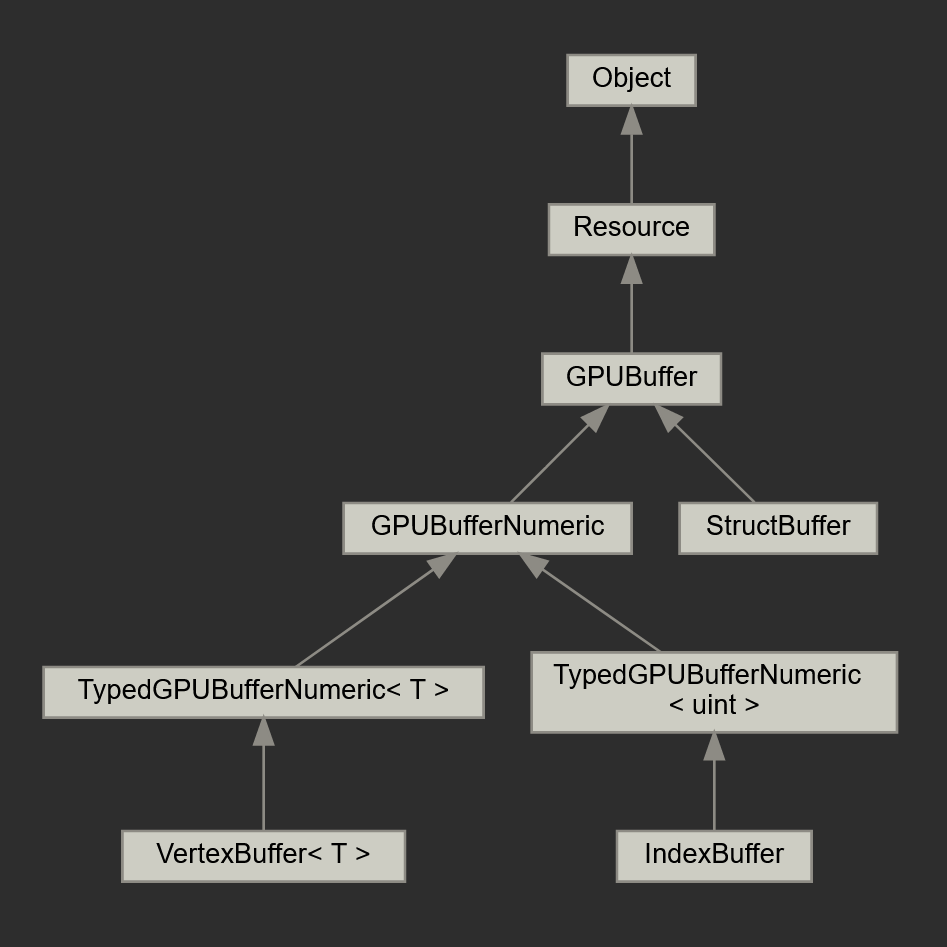
This furthermore shows that nap::VertexBuffer and nap::IndexBuffer share the same TypedGPUBufferNumeric<T> interface. These specializations are marked as VK_BUFFER_USAGE_VERTEX_BUFFER_BIT or VK_BUFFER_USAGE_INDEX_BUFFER_BIT on initialization making them available to be bound as attribute buffers in vertex shaders.
In the section 'Data', I demonstrate how to set up a struct buffer for particle simulation.
As with all things Vulkan; with great power comes great responsibility, which brings me to the topic of data synchronization. There are a few reasons we must be particularly wary of potential data synchronization hazards:
As a result, we must avoid potential data hazards ourselves. For instance, one operation may read from a buffer, while a preceding operation is actively writing to it. This is called a read-after-write hazard. Vice versa, a write-after-read hazard is when a buffer is written to while a preceding operations is still reading from it.
This is no different from the kind of synchronization problems we deal with when using the graphics pipeline for rendering. For this purpose, however, Vulkan offers specialized synchronization constructs such as renderpasses and subpasses. As compute dispatches include no such abstraction, the need for explicit synchronization arises (e.g. execution and memory barrier operations).
To alleviate the burden of synchronization, nap::ComputeComponent offers a simple general approach to protect your storage buffers from data hazards. The default implementation of onCompute() calls the protected member function insertBarriers() after vkCmdDispatch(). The function automatically places appropriate memory barriers based on usage properties of storage buffers as follows:
This fairly simple approach works as NAP imposes a strict command buffer submission order within a single frame of rendering: (1) compute, (2) headless - for offscreen render targets, (3) rendering - for window targets. This greatly reduces the complexity of synchronization. Here, we make the assumptions that any storage buffers present in the material instance will either be read in a subsequent render pass in the current frame, or accessed in a subsequent compute shader.
That pretty much concludes the overview of Compute. Next I'll show how to use the API in development.
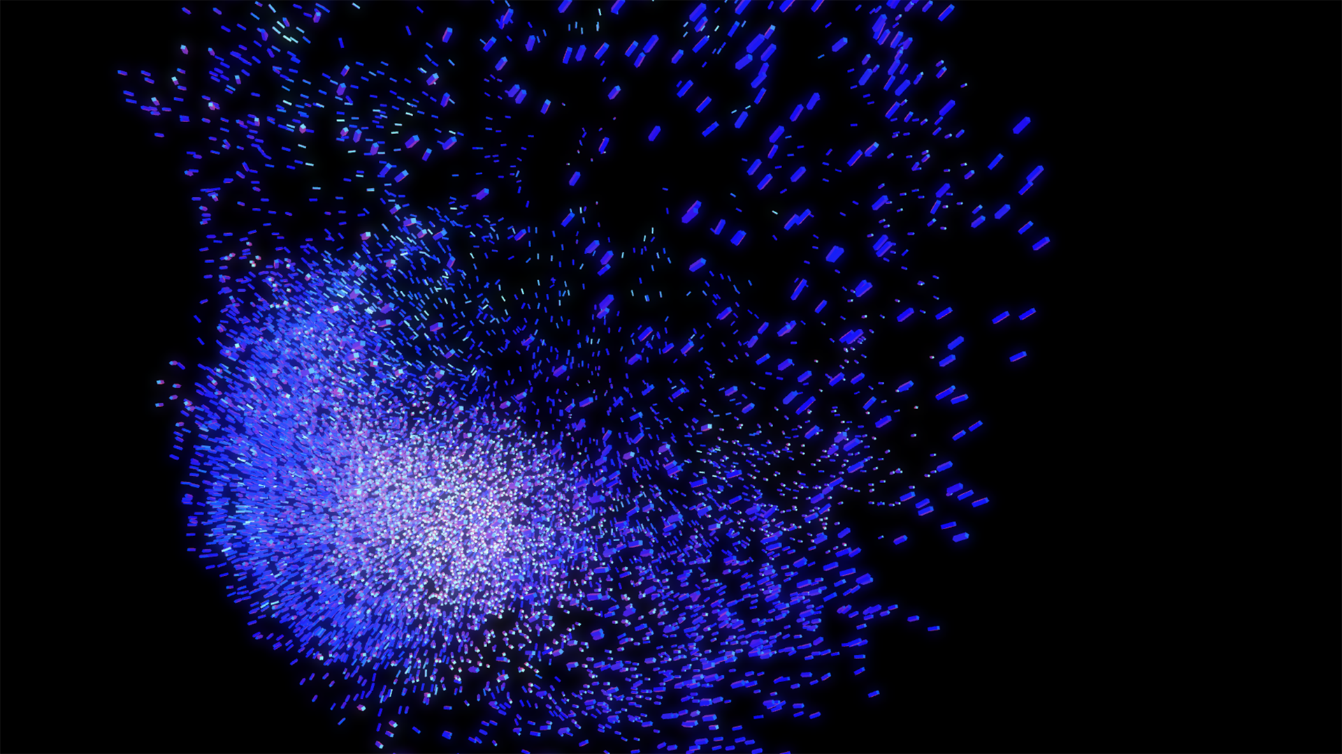
To demonstrate the possibilities of the new Compute update, I built the computeparticles and computeflocking demo's that ship with NAP. In this section I will go over some of the key elements that comprise the flocking demo and show they are set up. For an introduction to computational flocking systems, please refer to the seminal work by Reynolds: *"Reynolds, C. W. (1987, August). Flocks, herds and schools: A distributed behavioral model"*.
A flocking system consists of an arbitrary number of boids, each of which can freely move around the world with some kind of velocity. We can therefore formulate the data structure of a single boid transformation instance in a compute shader as follows:
Note that we use vec4 for each of our data members to fulfill GLSL's 16-byte alignment rules for scalars, vectors and array elements. Other than xyz-position and xyz-velocity, we encode orientation as a quaternion using four scalars (xyzw).
Our compute shader is called each frame and updates all boid transformations for the subsequent renderpass. In order to do this, we must evaluate the distances between all boids in the storage buffer (O^2). We use this brute-force approach for the sake of simplicity, but several interesting GPU acceleration structures and algorithms exist that will dramatically increase performance. Based on the boids in close enough proximity (mates) to another, we calculate three individual forces that dictate the flocking behavior; (1) alignment, (2) cohesion and (3) separation. The sum of these forces gives us the acceleration vector of a boid that we can use to update its velocity, orientation and position. You can view the full compute shader of the flocking demo, accompanied with explanatory comments, here.
Due to the asynchronous nature of Vulkan, we may be recording compute command for a future frame, while the last frame is still being processed. Therefore, we must avoid reading/writing to the same buffer in a single frame. We can overcome this problem by setting up a (double-buffered) bounce pass to update the boid transformations with two buffer bindings instead of one like so:
On the client side (CPU), we can toggle descriptor sets each frame to swap the underlying readonly and writeonly buffers using setBuffer().
What also works well to achieve this is using two instances of nap::ComputeComponent whose material instances have opposite in and out buffers, and alternating onCompute() between the two. This is the approach taken in the computeflocking demo.
Next, I'll show how to go about setting up resources for a flocking system setup in Napkin.
To declare a compute shader, you want to use nap::ComputeShaderFromFile.
Then, you can create a nap::ComputeMaterial and link the compute shader to its Shader property.
To create a storage buffer for the boid transforms, you want to use nap::StructBuffer. Then, declare the Boid struct element by creating an embedded nap::UniformStruct in the Element property. The GIF below only shows how to create the position member, but you will have to make sure to add velocity and orientation too.
Another very useful new feature that I haven't mentioned before are buffer fill policies. These are completely optional, but eliminate the need to fill the buffer on initialization manually. Here I create a nap::StructFillPolicy with a RandomFillPolicyVec4 for the position member. When linked to a buffer, it will generate an uniform random number (between LowerBound and UpperBound) for said member of each Boid element in the storage buffer (in this case, 10000 times).
Finally, we create a nap::ComputeComponent under a nap::Entity. Here, we make sure to reference the nap::ComputeMaterial we created earlier, and create a nap::BufferBindingStruct to reference our nap::StructBuffer. Make sure to do this for both BoidBuffer_In and BoidBuffer_Out.
That more or less concludes the resource setup for the compute shader.
As this example prepares a buffer for rendering we also have to make sure to bind the output storage buffer to our vertex shader so we can access the boid transformations for instanced rendering. To achieve this, we need custom onDraw() behavior and implement a class that inherits from nap::RenderableMeshComponent. We can then bind the storage buffer to the render material instance like as shown below, and call vkCmdDrawIndexed() with an instance count that is equal to the boid count.
Finally, in the vertex shader that renders the flock, we can use the built-in variable gl_InstanceIndex to lookup the correct boid transformation.
Hopefully this article helps to get a better understanding of the new Compute API. You can refer to our documentation to review compute-related resources and components, and further study the available demo's in the NAP repository. There is a bit more to the computeflocking demo than was discussed in this article, like a shared memory optimization and the use of specialization constants. The computeparticles is also worth checking out if you're interested in generating geometry in a compute shader, and binding storage buffers as vertex attributes for rendering. Make sure to reach out if you have any suggestions or happen to run into problems.
NAP Framework is open source software. Suggestions and contributions are welcome.
Lesley van Hoek | Software Engineer | NAP & NAP Labs
